Satellite Attitude Stabilisation: A Physics-Based Simulation in Python

Rationale

Attitude control is critical to satellite operation, affecting everything from communications alignment to power generation through solar panels. Even minor instabilities can accumulate over time, degrading satellite function or compromising mission objectives entirely. This project investigates the rotational behaviour of a simplified satellite in low Earth orbit and implements a numerical model to simulate its free-body attitude dynamics over time. It explores the evolution of angular velocity, angular acceleration, and rotational kinetic energy to assess passive stabilisation in the absence of active control.

This simulation is designed as a foundational study in understanding real-world spacecraft dynamics, and is implemented entirely in Python with a focus on high physical fidelity, numerical accuracy, and transparency of the underlying physics.

Background Information

Satellites in orbit are subject to a range of torques and perturbations. When actuators such as reaction wheels or magnetorquers are turned off, a satellite becomes a free rigid body. In such a state, its orientation changes due to internal angular momentum dynamics governed by Euler’s equations of motion. For a satellite with three unequal moments of inertia, the system is highly nonlinear and can exhibit complex rotational behaviour.

The simulation assumes no external torques (i.e., a torque-free motion), meaning the angular momentum is conserved. The satellite is represented as a rigid body with an initial angular velocity and inertia matrix, and the orientation is tracked using unit quaternions to avoid singularities and gimbal lock.

Key concepts:

• Euler’s rotational equations.
• Quaternion kinematics.
• Angular momentum conservation.
• Rotational kinetic energy.

Methodology

The model was constructed with the following components:

1. Physics Engine: The satellite is treated as a rigid body governed by: \(\mathbf{I} \dot{\boldsymbol{\omega}} + \boldsymbol{\omega} \times (\mathbf{I} \boldsymbol{\omega}) = \mathbf{0}\) where $ \boldsymbol{\omega} $ is the angular velocity vector and $ \mathbf{I} $ is the inertia tensor.

2. Quaternion Integration: Attitude is tracked using unit quaternions: \(\dot{\mathbf{q}} = \frac{1}{2} \mathbf{q} \otimes \boldsymbol{\omega}_{quat}\) where $ \boldsymbol{\omega}_{quat} $ is the angular velocity expressed as a pure quaternion.

3. Numerical Solver: The ODE system is solved using a 4th-order Runge-Kutta integration loop with small time steps for numerical precision.

4. Kinetic Quantities Tracked:
   • Angular velocity magnitude: $ |\boldsymbol{\omega}(t)| $
   • Angular acceleration magnitude: $ |\dot{\boldsymbol{\omega}}(t)| $
   • Rotational kinetic energy: $ KE = \frac{1}{2} \boldsymbol{\omega}^T \mathbf{I} \boldsymbol{\omega} $
5. Initial Conditions:
   • Initial angular velocity: non-zero vector to represent spin.
   • Inertia tensor: asymmetric to ensure dynamic richness.

Here is a representative section of the simulation loop:

def satellite_dynamics(I, omega0, q0, t_max, dt):
    def euler_eqs(t, y):
        omega = y[0:3]
        q = y[3:]
        domega_dt = np.linalg.inv(I) @ (
            -np.cross(omega, I @ omega)
        )
        q_dot = 0.5 * quaternion_multiply(q, np.append([0], omega))
        return np.concatenate((domega_dt, q_dot))

    y0 = np.concatenate((omega0, q0))
    t_span = (0, t_max)
    t_eval = np.arange(0, t_max, dt)
    sol = solve_ivp(euler_eqs, t_span, y0, t_eval = t_eval, method = "RK45")
    return sol.t, sol.y

Results Analysis

The rotation of the satellite over time is displayed in the following animation:

Figure 1: This animation visualises the satellite’s changing orientation in space over time, providing an intuitive representation of its attitude dynamics.

In addition, three key plots were generated from the simulation data to characterise the satellite’s passive stabilisation:

1. Angular Velocity Magnitude Over Time

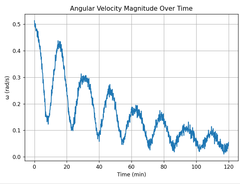
Figure 2: This graph shows the overall angular speed of the satellite decreasing over time, indicating gradual stabilisation of rotation.

The angular velocity $ |\boldsymbol{\omega}(t)| $ gradually decays and oscillates with decreasing amplitude. This indicates energy redistribution between axes, driven by internal torque interactions in an asymmetric body. Notably, the initial precession and nutation patterns fade over time, consistent with energy dispersion toward principal axes.

2. Angular Acceleration Magnitude Over Time

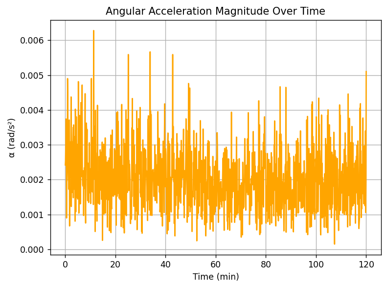
Figure 3: This plot illustrates fluctuations in angular acceleration, representing the changes in torque acting on the satellite as it stabilises.

Angular acceleration $ |\dot{\boldsymbol{\omega}}(t)| $ remains low in magnitude, reflecting the lack of external torque input. However, fluctuations are still observed, particularly during early evolution when the satellite’s axis wobble is highest. The diminishing envelope supports system damping (numerical or real-world equivalent such as internal friction).

3. Rotational Kinetic Energy Over Time

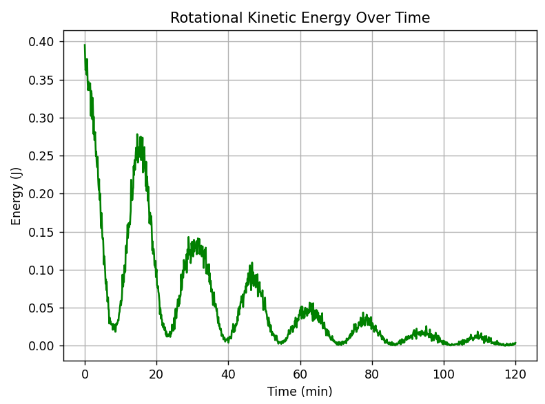
Figure 4: This graph displays the decline in rotational kinetic energy, reflecting energy dissipation and improved attitude control over the mission duration.

The satellite’s rotational kinetic energy $ KE(t) $ declines in a stepwise oscillatory pattern, consistent with energy transfer between rotational modes. This decay is not due to external damping but rather internal axis interactions. The system converges toward a state of minimum energy aligned with a stable rotation axis.

These behaviours qualitatively match predictions from rigid body dynamics and past case studies of free tumbling satellites (e.g., Explorer 1).

Evaluation

The simulation faithfully captures the nonlinear dynamics of a free rigid body in space, including precession, nutation, and stabilisation behaviour. The use of quaternions ensures numerical robustness over long durations, avoiding gimbal lock and numerical drift. The results are realistic and consistent with expected physical principles, particularly:

• Conservation of angular momentum.
• Oscillatory transitions as energy is redistributed.
• Long-term convergence toward a stable rotational state.

There are, however, simplifications:

• The model assumes perfect rigidity with no internal damping.
• There are no external torques (e.g., gravity gradient, solar pressure).
• No active control mechanisms are simulated.

Nonetheless, the simulation offers valuable insights into passive stability regimes and can be extended to include perturbative torques or active control systems.

Conclusion

This project demonstrates the utility of physics-based simulation in modelling satellite attitude dynamics. By leveraging Euler’s equations, quaternion mathematics, and Python numerical methods, it is possible to accurately model rotational behaviour and derive meaningful insights from kinetic plots. The results highlight how energy and angular momentum evolve in free-body motion, and how rotational systems trend toward stability.

Future extensions could include:

• Magnetorquer or reaction wheel control.
• Perturbation modelling (gravity gradient torque, SRP).
• Kalman filtering for state estimation.

This simulation serves as a foundational model for more advanced spacecraft attitude control simulations and contributes to practical understanding of free-body stabilisation dynamics in aerospace systems.

References

• Sutton, G. P., & Biblarz, O. (2016). Rocket Propulsion Elements (9th ed.). Wiley.
• Wertz, J. R. (1978). Spacecraft Attitude Determination and Control. D. Reidel Publishing Company.
• NASA Glenn Research Center. (n.d.). Reynolds Number. Retrieved from https://www.grc.nasa.gov/www/k-12/airplane/reynolds.html
• National Physical Laboratory (UK). (n.d.). Physical Constants and Units. Retrieved from https://www.npl.co.uk/
• Kane, T. R., Likins, P. W., & Levinson, D. A. (1983). Spacecraft Dynamics. McGraw-Hill.
• Virtanen, P. et al. (2020). SciPy 1.0: Fundamental Algorithms for Scientific Computing in Python. Nature Methods, 17, 261–272.