Aerodynamic Shape Optimisation Using Machine Learning and Evolutionary Algorithms

Rationale

In mechatronic and aerospace design, aerodynamic efficiency is a critical determinant of performance, fuel consumption, and thus emissions. Minimising aerodynamic drag has been a long-term focus in engineering disciplines due to its consequences on energy efficiency and operating costs. However, manual optimisation of complex shapes remains time-consuming and limited by human intuition.

This project investigates the utilisation of evolutionary algorithms to autonomously optimise a three-dimensional axisymmetric object’s geometry to reduce its aerodynamic drag. By simulating 1000 generations of Differential Evolution followed by 1000 iterations of Covariance Matrix Adaptation Evolution Strategy (CMA-ES), the programme aims to refine shapes using physics-informed fitness evaluations. The objective of this programme is to demonstrate the applicability of machine learning in solving real-world engineering problems involving fluid dynamics, stability, and form efficiency.

Background Information

Aerodynamic Drag

Drag is the resistance force acting opposite to the motion of an object moving through a fluid, such as air. It is composed of several components:

• Form Drag (Pressure Drag) arises from the shape of the object and the pressure differential between the front and rear surfaces.
• Skin Friction Drag is caused by viscous shear stresses in the boundary layer of air along the surface.
• Base Drag occurs at the rear of bluff bodies due to flow separation.
• Induced Drag arises from lift generation, albeit minimal for streamlined bodies.
• Wake Drag is associated with turbulence behind the object.

These drag forces are typically modelled using:

\[D = \frac{1}{2} \rho v^2 C_d A\]

Where:

• $D$ is the drag force (N)
• $\rho$ is the air density (kg/m³)
• $v$ is the velocity (m/s)
• $C_d$ is the drag coefficient (dimensionless)
• $A$ is the frontal area (m²)

Reynolds Number

The Reynolds number, given by:

\[Re = \frac{\rho v L}{\mu}\]

quantifies the flow regime, separating laminar and turbulent conditions. The critical Reynolds number of $5 \times 10^5$ is used to switch between laminar and turbulent skin friction formulations.

Evolutionary Algorithms

Evolutionary algorithms are heuristic optimisation techniques inspired by natural selection. Two methods are used in this study:

• Differential Evolution (DE) iteratively evolves a population of candidate solutions by combining existing candidates to generate new ones, selecting those with better performance.
• CMA-ES (Covariance Matrix Adaptation Evolution Strategy) refines solutions by sampling from a multivariate Gaussian distribution and updating its covariance matrix based on successful solutions.

These algorithms require an objective function to evaluate each solution, in this case, total aerodynamic drag.

Geometry Modelling

The object is defined by a set of control points describing half of its side profile. These points are interpolated using cubic splines. The resulting profile is revolved to estimate frontal area, wetted area, and volume. The shape is then assessed based on fluid dynamic parameters.

Additional Physics

The simulation incorporates additional physical phenomena:

• Compressibility Corrections for Mach numbers above 0.3 using the Prandtl-Glauert transformation.
• Stability Margins calculated using an estimate of the centre of mass and centre of pressure.
• Ground Effect reduces form drag when near the surface.
• Surface Roughness adds a correction factor to simulate real-world conditions.

Methodology

Constants and Assumptions

The following constants and assumptions were applied:

• Velocity: 30 m/s
• Target Mass: 500 kg
• Max Side Profile Length: 3.0 m
• Max Frontal Profile Length: 1.0 m
• Object Density: 500 kg/m³
• Air density: 1.225 kg/m³ (at sea level)
• Surface roughness coefficient: 1.05
• Lift coefficient: 0.05 (to simulate mild induced drag)
• Ground effect applied below 0.5 m altitude

Simulation Procedure

The simulation proceeds as follows:

1. Initial Geometry Generation:

def generate_profile(control_points, length, num_points = 500):
    xs_control = np.linspace(0, length, NUM_CONTROL_POINTS)
    ys_control = np.abs(control_points)
    ys_control[0] = ys_control[-1] = 0
    interp_func = interp1d(xs_control, ys_control, kind = "cubic")
    xs = np.linspace(0, length, num_points)
    ys = interp_func(xs)
    return xs, ys

The ML algorithm modifies the shape by adjusting a vector of parameters that includes:

• Eight vertical control point values, which define the curvature of the side profile using cubic spline interpolation. These values control the local radius along the object’s length, effectively shaping the profile’s smoothness, thickness distribution, and taper.
• Total side profile length, which determines the overall body length of the shape and influences the fineness ratio.
• Frontal profile length (width), which defines the elliptical diameter of the object’s cross-section and directly affects the frontal area.

These twelve parameters allow the ML algorithm to explore a wide design space of slender, symmetrical bodies while ensuring that the shape remains smooth and physically realistic. Although, the three-dimensional shape remains incredibly rudimentary when compared to the real-world applications of drag reduction.

2. Drag Evaluation: The main function computes:

• Frontal and wetted surface area.
• Reynolds number and skin friction.
• Volume and mass penalties.
• Smoothness and stability penalties.
• Total drag (sum of all components).

def evaluate_drag(params, velocity, target_mass):
    ...

3. Optimisation:

• Differential Evolution runs for 1000 generations.
• CMA-ES uses the DE result as a seed and performs 1000 iterations.

result_de = differential_evolution(...)
es = cma.CMAEvolutionStrategy(result_de.x.tolist(), 0.02)
es.optimize(lambda p: evaluate_drag(p, velocity, target_mass, max_length, max_front_length), iterations = 1000)

4. Logging and Visualisation: Each generation’s data is stored in a DataFrame and visualised through:

• Side and frontal profile plots, to determine the accuracy of the programme.
• Drag versus generation graph, to investigate the impact of each subsequent generation on drag.

Results Analysis

Final Output

After 2000 total optimisation steps (1000 DE + 1000 CMA-ES), the best solution appeared in Generation 990.

Parameter	Value
Generation	990
Final Drag (N)	169.21
Velocity (m/s)	30.0
Mass (kg)	500.0
Length (m)	3.0
Frontal Width (m)	0.77
Frontal Length (m)	1.0

Table 1: Fully optimised parameters of the shape at its most optimal generation.

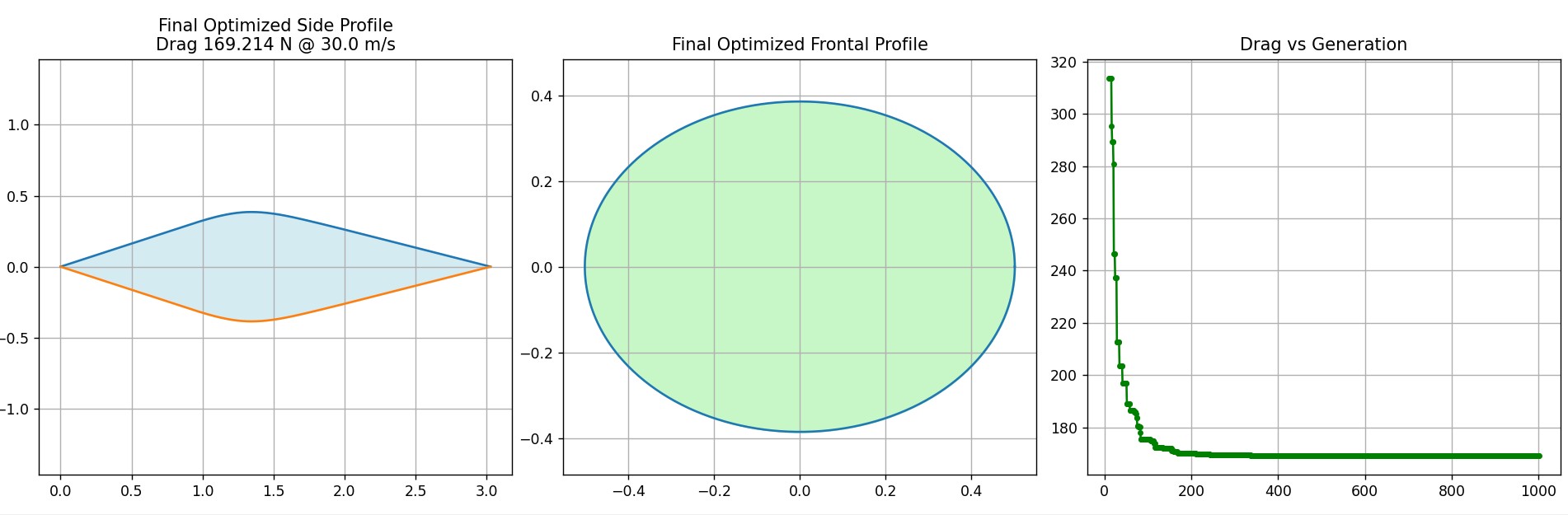
Figure 1: Final profile of optimised shape showing smooth axisymmetric curvature, and a graph displaying the change in drag over each generation.

Figure 2: Drag evolution over 1000 generations of Differential Evolution and CMA-ES.

Side and Frontal Profile

The final side profile exhibits a smooth, continuous curvature that peaks at the midsection and tapers symmetrically towards the nose and tail (a symmetrical teardrop shape). This streamlined geometry minimises pressure drag by delaying flow separation, particularly at higher velocities where adverse pressure gradients are more influential. The use of cubic spline interpolation across eight control points ensures a high degree of shape control without introducing abrupt surface changes, which would otherwise elevate form drag.

The frontal profile is elliptical, a shape known to reduce stagnation pressure at the leading edge while also constraining frontal area. This elliptical cross-section balances structural efficiency and aerodynamic performance, producing a compact footprint (0.7707 m diameter) relative to the overall length (3.0 m). Note that the frontal profile is a 2-dimensional representation of how the shape would appear from the front, thus displaying the shape’s largest surface area from the frontal plane.

Together, these forms suggest a high fineness ratio design that is representative of real-world applications such as drop tanks, unmanned aerial vehicles, or missile fuselages, where low drag and dynamic stability are critical.

Drag vs Generation

As the number of generations increases from 0 to 50, the drag decreases significantly in decreasing increment, which is due to the elimination of grossly inefficient shapes early on. Subsequent refinements were smaller, with diminishing returns as the algorithms approached local minima. Onwards from generation 50, the data displays an inverse proportionality, as the drag decreases negligibly and plateaus. From here, the CMA-ES began optimisation within an already narrow solution space.

This behaviour reflects a realistic optimisation curve, where coarse improvements precede subtle, high-fidelity tuning. Evidently, only 400 generations are necessary for a decently accurate drag reduction to occur, but extremely precise operations may require more. Importantly, skipping the first five generations from the plot improves readability by excluding early-stage outliers.

Evaluation

Accuracy and Limitations

• The drag models are simplified, lacking vortex shedding, turbulent wake prediction, or 3D finite element resolution.
• Revolved axisymmetric bodies do not capture features like wings, vents, or sharp edges.
• No structural or thermal constraints were considered beyond stability margins.
• Air density remains fixed, without altitude or temperature variation beyond a single exponential decay.

Suggested Improvements

1. Incorporate Real CFD Libraries such as OpenFOAM or PyFoam for detailed pressure field evaluation.
2. Thermal Constraints to simulate high-speed heating or radiative cooling.
3. Material Strength Models to introduce minimum wall thickness or failure stress constraints.
4. Stochastic Wind Conditions to evaluate shape performance under varying angles of attack or gusts.
5. Multifidelity Models where rough analytical models guide early optimisation, switching to CFD later.

Conclusion

This project demonstrated the employment of evolutionary algorithms to optimise a superficial three-dimensional shape for minimal aerodynamic drag. By integrating mathematical modelling, physics-based penalty functions, and machine learning-based search, the program effectively identified efficient geometries under realistic constraints. The success of this approach in a simplified domain provides a valuable stepping stone toward more sophisticated design tools in aerospace, automotive, and civil engineering contexts. Continued development, particularly through integration with CFD and real-world testing, would significantly enhance the fidelity and applicability of such simulations.

References

• Anderson, J. D. (2010). Fundamentals of Aerodynamics. McGraw-Hill.
• Hansen, N. (2006). The CMA Evolution Strategy: A Comparing Review.
• White, F. M. (2011). Fluid Mechanics. McGraw-Hill.
• NASA Glenn Research Center. (2022). Drag Equation. https://www.grc.nasa.gov