<?xml version="1.0" encoding="utf-8"?><feed xmlns="http://www.w3.org/2005/Atom" ><generator uri="https://jekyllrb.com/" version="3.10.0">Jekyll</generator><link href="https://james-brandt.github.io/feed.xml" rel="self" type="application/atom+xml" /><link href="https://james-brandt.github.io/" rel="alternate" type="text/html" /><updated>2025-12-23T22:44:20+10:00</updated><id>https://james-brandt.github.io/feed.xml</id><title type="html">Projects by James Brandt</title><subtitle>Explore personal, experimental, and in-progress projects in programming, AI, and engineering.</subtitle><author><name>James Brandt</name></author><entry><title type="html">Quantifying the Impact of Solar Activity on Satellite Re-Entry Rates</title><link href="https://james-brandt.github.io/satellite-entry-rates/" rel="alternate" type="text/html" title="Quantifying the Impact of Solar Activity on Satellite Re-Entry Rates" /><published>2025-12-20T00:00:00+10:00</published><updated>2025-12-20T00:00:00+10:00</updated><id>https://james-brandt.github.io/satellite-entry-rates</id><content type="html" xml:base="https://james-brandt.github.io/satellite-entry-rates/"><![CDATA[<p>Work in progress…</p>]]></content><author><name>James Brandt</name></author><summary type="html"><![CDATA[An empirical analysis using orbital and space weather data to compare satellite re-entry rates to solar activity.]]></summary></entry><entry><title type="html">Optimising Brake Bias in Formula 1: A Physics-Based Mini-Project</title><link href="https://james-brandt.github.io/brake-bias-optimiser/" rel="alternate" type="text/html" title="Optimising Brake Bias in Formula 1: A Physics-Based Mini-Project" /><published>2025-11-12T00:00:00+10:00</published><updated>2025-11-12T00:00:00+10:00</updated><id>https://james-brandt.github.io/brake-bias-optimiser</id><content type="html" xml:base="https://james-brandt.github.io/brake-bias-optimiser/"><![CDATA[<h2 id="rationale">Rationale</h2>

<p>Dynamic brake proportioning (commonly referred to as brake bias) is essential for optimising F1 lap performance. This precise calibration of the braking force between the front and rear axles is critical for vehicle stability, contributing to time gains. Drivers adjust their brake bias mid-lap to compensate for fluctuating vehicle speed, variations in corner geometry, and tyre conditions.</p>

<p>Determining the optimal brake bias for specific corners and conditions requires quantitative data from real vehicle testing. Thus, the purpose of an optimised mathematical model is to be utilised as a baseline for teams during testing and practise sessions. This project largely explores avoiding the requirement of computational simulation software such as CFD — which has a restricted number of hours of usage per FIA regulations — by simplifying complex concepts into functions and equations. Rudimentary Python code further automates and accelerates these calculations, allowing the user to manually input the conditions of a specific corner to output the calculated optimal brake bias.</p>

<h2 id="background-information">Background Information</h2>

<h3 id="the-physics-of-brake-bias">The Physics of Brake Bias</h3>

<p>Brake bias defines the ratio of total braking force distributed between the front and rear axles (for example, 55% brake bias indicates that 55% of the deceleration force is distributed to the front of the vehicle). The requirement for front-axle bias is a necessity due to the following factors:</p>

<ul>
  <li>
    <p>Longitudinal Load Transfer: Upon braking, the normal load on the front tyres swiftly increases while the load on the rear diminishes, due to the inertia generated by the vehicle’s rapid deceleration.</p>
  </li>
  <li>
    <p>Friction Ellipse Constraint: A tyre can generate longitudinal (braking) and lateral (cornering) forces simultaneously, but both cannot be maximised at once. That is, tyres have a certain capacity for forces that must be shared longitudinally and laterally.</p>
  </li>
  <li>
    <p>Stability Constraint: The optimal bias must be precisely constrained to maintain stability. Excessive front bias increases the risks of lock-ups, while excessive rear bias induces rear wheel lock-ups, and increases the chance of the vehicle spinning out. A 90% front to 10% rear bias would violate this constraint, for example.</p>
  </li>
</ul>

<p>The optimal bias is the precise point wherein both axles operate at their maximum available friction limit.</p>

<h3 id="mathematical-model">Mathematical Model</h3>

<p>This mathematical model employs the following equations and simplifications:</p>

<ul>
  <li>
    <p>The vehicle mass $m$, wheelbase $L$, centre-of-gravity (CoG) height $h_{cg}$, and front-wheel CoG distance $a_{cg}$ are fixed.</p>
  </li>
  <li>
    <p>Static normal loads on front and rear axles are given by the simple lever arm of weight distribution:</p>
  </li>
</ul>

\[N_{f,static} = m \times g \times \frac{L - a_{cg}}{L}, N_{r,static} = m \times g \times \frac{a_{cg}}{L}\]

<ul>
  <li>Under braking deceleration $a_{x}$ the longitudinal transfer is:</li>
</ul>

\[\Delta N = \frac{m \times a_{x} \times h_{cg}}{L}\]

<ul>
  <li>
    <p>Aero downforce on each axle is approximated as $D = \frac{1}{2} \rho A C_{l} v^{2}$ , separated into front and rear fractions.</p>
  </li>
  <li>
    <p>Lateral acceleration $a_{y}$ is derived from corner radius $R$ and entry speed $v$: $a_{y} = \frac{v^{2}}{R}$. That gives lateral force total $F_{y,total} = m \times a_{y}$.</p>
  </li>
  <li>
    <p>For each axle, the remaining braking (longitudinal) capacity is computed using a simplified friction circle (where $\mu$ is peak tyre friction assumed equal front/rear in this model):</p>
  </li>
</ul>

\[F_{f,max} = \sqrt{(\mu \times N)^{2} - (F_{y,used})^{2}}\]

<ul>
  <li>
    <p>The total braking force required: $F_{x,total} = m \times a_{x}$.</p>
  </li>
  <li>
    <p>Therefore, optimum front bias fraction is:</p>
  </li>
</ul>

\[bias_{front} = \frac{F_{x,front,max}}{F_{x,front,max} + F_{x,rear,max}}\]

<ul>
  <li>The search range (for realism and to ensure vehicular stability) is set to be between 45% and 60% front.</li>
</ul>

<h3 id="assumptions-inclusions-and-omissions">Assumptions, Inclusions and Omissions</h3>
<ul>
  <li>
    <p>The following factors are omitted: a variation in friction between the front and rear tyres, tyre compound differences, the effects of weight transfer (pitch or roll), hybrid powertrain regeneration effects, and driver behaviour (whether the driver employs trail braking, or traditionally brakes and then turns).</p>
  </li>
  <li>
    <p>It is assumed that the vehicle is at a constant entry velocity, applying a constant deceleration before cornering. Only a single corner is modelled, though the exact conditions would be modifiable.</p>
  </li>
  <li>
    <p>The model neglects engine braking, temperature changes, tyre wear, path variation and bumpiness.</p>
  </li>
</ul>

<h2 id="methodology">Methodology</h2>

<h3 id="code-overview">Code Overview</h3>
<p>Below are excerpts of some important Python functions used in the project.</p>

<div class="language-python highlighter-rouge"><div class="highlight"><pre class="highlight"><code><span class="c1"># Static normal loads
</span><span class="k">def</span> <span class="nf">static_normal_loads</span><span class="p">(</span><span class="n">mass</span><span class="p">,</span> <span class="n">gravity</span><span class="p">,</span> <span class="n">load</span><span class="p">,</span> <span class="n">a_cg</span><span class="p">):</span>
    <span class="n">Nf</span> <span class="o">=</span> <span class="n">mass</span> <span class="o">*</span> <span class="n">gravity</span> <span class="o">*</span> <span class="p">(</span><span class="n">load</span> <span class="o">-</span> <span class="n">a_cg</span><span class="p">)</span> <span class="o">/</span> <span class="n">load</span>
    <span class="n">Nr</span> <span class="o">=</span> <span class="n">mass</span> <span class="o">*</span> <span class="n">gravity</span> <span class="o">*</span> <span class="p">(</span><span class="n">a_cg</span><span class="p">)</span> <span class="o">/</span> <span class="n">load</span>
    <span class="k">return</span> <span class="n">Nf</span><span class="p">,</span> <span class="n">Nr</span>

<span class="c1"># Longitudinal load transfer
</span><span class="k">def</span> <span class="nf">longitudinal_load_transfer</span><span class="p">(</span><span class="n">mass</span><span class="p">,</span> <span class="n">ax_brake</span><span class="p">,</span> <span class="n">h_cg</span><span class="p">,</span> <span class="n">load</span><span class="p">):</span>
    <span class="k">return</span> <span class="n">mass</span> <span class="o">*</span> <span class="n">ax_brake</span> <span class="o">*</span> <span class="n">h_cg</span> <span class="o">/</span> <span class="n">load</span>

<span class="c1"># Aero downforce functions
</span><span class="k">def</span> <span class="nf">Df_front</span><span class="p">(</span><span class="n">velocity</span><span class="p">):</span>
    <span class="k">return</span> <span class="mf">0.5</span> <span class="o">*</span> <span class="n">rho</span> <span class="o">*</span> <span class="n">area</span> <span class="o">*</span> <span class="n">Cl_front</span> <span class="o">*</span> <span class="n">velocity</span><span class="o">**</span><span class="mi">2</span>

<span class="k">def</span> <span class="nf">Df_rear</span><span class="p">(</span><span class="n">velocity</span><span class="p">):</span>
    <span class="k">return</span> <span class="mf">0.5</span> <span class="o">*</span> <span class="n">rho</span> <span class="o">*</span> <span class="n">area</span> <span class="o">*</span> <span class="n">Cl_rear</span>  <span class="o">*</span> <span class="n">velocity</span><span class="o">**</span><span class="mi">2</span>

<span class="c1"># Friction circle remaining braking force
</span><span class="k">def</span> <span class="nf">friction_circle_remaining_longitudinal</span><span class="p">(</span><span class="n">mu</span><span class="p">,</span> <span class="n">N_axle</span><span class="p">,</span> <span class="n">Fy_used</span><span class="p">):</span>
    <span class="n">term</span> <span class="o">=</span> <span class="p">(</span><span class="n">mu</span> <span class="o">*</span> <span class="n">N_axle</span><span class="p">)</span><span class="o">**</span><span class="mi">2</span> <span class="o">-</span> <span class="n">Fy_used</span><span class="o">**</span><span class="mi">2</span>
    <span class="k">if</span> <span class="n">term</span> <span class="o">&lt;</span> <span class="mi">0</span><span class="p">:</span>
        <span class="k">return</span> <span class="mf">0.0</span>
    <span class="k">return</span> <span class="n">math</span><span class="p">.</span><span class="n">sqrt</span><span class="p">(</span><span class="n">term</span><span class="p">)</span>

<span class="c1"># Compute brake bias
</span><span class="k">def</span> <span class="nf">compute_brake_bias_from_radius</span><span class="p">(</span><span class="n">v_entry</span><span class="p">,</span> <span class="n">R_corner</span><span class="p">,</span> <span class="n">ax_brake</span><span class="p">):</span>
    <span class="n">ay_target</span> <span class="o">=</span> <span class="n">v_entry</span><span class="o">**</span><span class="mi">2</span> <span class="o">/</span> <span class="n">R_corner</span>
    <span class="k">return</span> <span class="n">compute_brake_bias</span><span class="p">(</span><span class="n">v_entry</span> <span class="o">=</span> <span class="n">v_entry</span><span class="p">,</span> <span class="n">ay_target</span> <span class="o">=</span> <span class="n">ay_target</span><span class="p">,</span> <span class="n">ax_brake</span> <span class="o">=</span> <span class="n">ax_brake</span><span class="p">)</span>
</code></pre></div></div>

<h3 id="full-process-and-experimentation">Full Process and Experimentation</h3>
<ol>
  <li>Define car parameters (mass, geometry, aero coefficients, tyre friction coefficient, brake bias search range).</li>
  <li>Build the model functions for load transfer, aero load, lateral force split, braking capacity per axle.</li>
  <li>For each trial input (entry speed $v$, corner radius $R$, deceleration $a_{x}$) compute optimum front bias fraction.</li>
  <li>Compare experimental brake bias values to predicted values.</li>
</ol>

<h2 id="results--analysis">Results &amp; Analysis</h2>

<h3 id="experimental-trials">Experimental Trials</h3>

<p>Three distinct trials were tested to evaluate the accuracy and precision of the model:</p>
<ol>
  <li>Trial A: Heavy braking zone from high speed into tight corner. $v_{entry}$ = 90m/s, $R_{corner}$ = 60m, $a_{x,brake}$ = 4.5g.</li>
  <li>Trial B: Medium braking zone, moderate speed and radius. $v_{entry}$ = 70m/s, $R_{corner}$ = 120m, $a_{x,brake}$ = 3.5g.</li>
  <li>Trial C: Light braking into flowing corner. $v_{entry}$ = 60m/s, $R_{corner}$ = 200m, $a_{x,brake}$ = 2.5g.</li>
</ol>

<table>
  <thead>
    <tr>
      <th>Trial</th>
      <th>Experimental Bias (front %)</th>
      <th>Expected Bias (front %)</th>
      <th>% Difference</th>
    </tr>
  </thead>
  <tbody>
    <tr>
      <td>A</td>
      <td>50.00 %</td>
      <td>55.0 %</td>
      <td>−9.09 %</td>
    </tr>
    <tr>
      <td>B</td>
      <td>62.01 %</td>
      <td>60.0 %</td>
      <td>+3.35 %</td>
    </tr>
    <tr>
      <td>C</td>
      <td>59.73 %</td>
      <td>60.0 %</td>
      <td>−0.45 %</td>
    </tr>
  </tbody>
</table>

<p class="text-center" style="font-size:0.65rem;">
  <strong>Table 1:</strong> Table of results of the three test trials, including the percentage difference between the expected bias values and the experimental bias values. It is important to note that the expected values are somewhat contextual, and affected by factors that have been omitted from this model. They are a general indication of where the experimental values should lie. 
</p>

<h3 id="interpretation">Interpretation</h3>
<ul>
  <li>The results show that the model produces different optimal biases for the different corner scenarios, proving a degree of reliability though not indicative of its accuracy.</li>
  <li>Trial A being at 50% frontal brake bias highlights a scenario with relatively lesser deceleration, causing the front bias requirement to decrease. This bias is somewhat lower than the expected5 55-60% for heavy braking. Although, this value is not a strictly inaccurate, as 50% bias may be employed under certain conditions.</li>
  <li>Trial B’s 62% frontal brake bias may demonstrate that the input values represent an unusually heavy braking zone, or that the model possesses a degree of inaccuracy under higher braking conditions.</li>
  <li>Trial C’s 59.73% frontal brake bias lies within the typical 60% front range expected for this turn. It is an indication of accuracy for this specific trial.</li>
</ul>

<h3 id="real-world-comparison">Real-World Comparison</h3>
<p>Because there are no publicly published ideal bias percentages for specific track corners, the absolute accuracy of the model cannot be validated against real telemetry. Instead, the expected values utilised from published simulation data intends to highlight whether the simulation data is within an appropriate range, the variations in brake bias is consistent, and the trend is accurate.</p>

<h2 id="evaluation">Evaluation</h2>

<h3 id="strengths">Strengths</h3>
<ul>
  <li>
    <p>The results are reasonable, mostly accurate, and vary with input corner severity, indicating a successful correlation between the input variables and the brake bias ratio.</p>
  </li>
  <li>
    <p>The model captures key physics concepts in Formula One: deceleration, weight shift, tyre load, and friction.</p>
  </li>
</ul>

<h2 id="weaknesses">Weaknesses</h2>
<ul>
  <li>
    <p>The tyre model is very simplified through its uniform front and rear friction and its lack in tyre variation.</p>
  </li>
  <li>
    <p>Braking via hybrid energy recovery (which affect rear braking load in modern Formula One cars) is omitted. The rear braking in Formula One is partly handled by engine braking and the ERS system, so the simple rear braking force assumption is an approximation when the hybrid powertrain is considered.</p>
  </li>
  <li>
    <p>The scenario inputs were not tied to publicly-verified data with known bias values. Without actual bias values for those corners, the model cannot be truly validated.</p>
  </li>
</ul>

<h2 id="conclusion">Conclusion</h2>

<p>This mini-project has shown that by utilising the fundamental physics of braking, weight transfer, lateral versus longitudinal forces, and aerodynamic load, one can program a moderately accurate model to predict optimal brake bias for a Formula One car in a cornering-braking scenario. Although the model cannot be validated against published corner-specific bias values (which are not publicly available), the results demonstrate credibility: they sit within the expected range (50% to 60% front), and they illustrate the expected correlation between the input variables and the output brake bias.</p>

<h2 id="references">References</h2>

<ul>
  <li>Flow Racers. (2023, April 4). What is brake bias in F1? (Fully explained). FlowRacers. <a href="https://www.flowracers.com/blog/f1-brake-bias/">https://www.flowracers.com/blog/f1-brake-bias/</a></li>
  <li>Formulapedia. (2022, October 2). What is brake balance in F1? (Brake bias explained). Formulapedia. <a href="https://www.formulapedia.com/brake-balance-in-f1/">https://www.formulapedia.com/brake-balance-in-f1/</a></li>
  <li>Las Motorsport. (2024). Brake balance in F1: What you need to know. Las Motorsport. <a href="https://las-motorsport.com/f1/blog/brake-balance-in-f1-what-you-need-to-know/3997/">https://las-motorsport.com/f1/blog/brake-balance-in-f1-what-you-need-to-know/3997/</a></li>
  <li>Mercedes-AMG Petronas F1. (n.d.). Formula One brake systems, explained! Mercedes-AMG Petronas F1 Team. <a href="https://www.mercedesamgf1.com/news/formula-one-brake-systems-explained/">https://www.mercedesamgf1.com/news/formula-one-brake-systems-explained/</a></li>
</ul>]]></content><author><name>James Brandt</name></author><summary type="html"><![CDATA[Modelling and optimising front-axle brake bias for F1-style corner entries using vehicle dynamics and simulation-based code.]]></summary></entry><entry><title type="html">Satellite Attitude Stabilisation: A Physics-Based Simulation in Python</title><link href="https://james-brandt.github.io/satellite-attitude-stabilisation/" rel="alternate" type="text/html" title="Satellite Attitude Stabilisation: A Physics-Based Simulation in Python" /><published>2025-07-18T00:00:00+10:00</published><updated>2025-07-18T00:00:00+10:00</updated><id>https://james-brandt.github.io/satellite-attitude-stabilisation</id><content type="html" xml:base="https://james-brandt.github.io/satellite-attitude-stabilisation/"><![CDATA[<h2 id="rationale">Rationale</h2>

<p>Attitude control is critical to satellite operation, affecting everything from communications alignment to power generation through solar panels. Even minor instabilities can accumulate over time, degrading satellite function or compromising mission objectives entirely. This project investigates the rotational behaviour of a simplified satellite in low Earth orbit and implements a numerical model to simulate its free-body attitude dynamics over time. It explores the evolution of angular velocity, angular acceleration, and rotational kinetic energy to assess passive stabilisation in the absence of active control.</p>

<p>This simulation is designed as a foundational study in understanding real-world spacecraft dynamics, and is implemented entirely in Python with a focus on high physical fidelity, numerical accuracy, and transparency of the underlying physics.</p>

<h2 id="background-information">Background Information</h2>

<p>Satellites in orbit are subject to a range of torques and perturbations. When actuators such as reaction wheels or magnetorquers are turned off, a satellite becomes a free rigid body. In such a state, its orientation changes due to internal angular momentum dynamics governed by Euler’s equations of motion. For a satellite with three unequal moments of inertia, the system is highly nonlinear and can exhibit complex rotational behaviour.</p>

<p>The simulation assumes no external torques (i.e., a torque-free motion), meaning the angular momentum is conserved. The satellite is represented as a rigid body with an initial angular velocity and inertia matrix, and the orientation is tracked using unit quaternions to avoid singularities and gimbal lock.</p>

<p>Key concepts:</p>
<ul>
  <li>Euler’s rotational equations.</li>
  <li>Quaternion kinematics.</li>
  <li>Angular momentum conservation.</li>
  <li>Rotational kinetic energy.</li>
</ul>

<h2 id="methodology">Methodology</h2>

<p>The model was constructed with the following components:</p>

<ol>
  <li>
    <p><strong>Physics Engine</strong>: The satellite is treated as a rigid body governed by:
\(\mathbf{I} \dot{\boldsymbol{\omega}} + \boldsymbol{\omega} \times (\mathbf{I} \boldsymbol{\omega}) = \mathbf{0}\)
where $ \boldsymbol{\omega} $ is the angular velocity vector and $ \mathbf{I} $ is the inertia tensor.</p>
  </li>
  <li>
    <p><strong>Quaternion Integration</strong>: Attitude is tracked using unit quaternions:
\(\dot{\mathbf{q}} = \frac{1}{2} \mathbf{q} \otimes \boldsymbol{\omega}_{quat}\)
where $ \boldsymbol{\omega}_{quat} $ is the angular velocity expressed as a pure quaternion.</p>
  </li>
  <li>
    <p><strong>Numerical Solver</strong>: The ODE system is solved using a 4th-order Runge-Kutta integration loop with small time steps for numerical precision.</p>
  </li>
  <li><strong>Kinetic Quantities Tracked</strong>:
    <ul>
      <li>Angular velocity magnitude: $ |\boldsymbol{\omega}(t)| $</li>
      <li>Angular acceleration magnitude: $ |\dot{\boldsymbol{\omega}}(t)| $</li>
      <li>Rotational kinetic energy: $ KE = \frac{1}{2} \boldsymbol{\omega}^T \mathbf{I} \boldsymbol{\omega} $</li>
    </ul>
  </li>
  <li><strong>Initial Conditions</strong>:
    <ul>
      <li>Initial angular velocity: non-zero vector to represent spin.</li>
      <li>Inertia tensor: asymmetric to ensure dynamic richness.</li>
    </ul>
  </li>
</ol>

<p>Here is a representative section of the simulation loop:</p>

<div class="language-python highlighter-rouge"><div class="highlight"><pre class="highlight"><code><span class="k">def</span> <span class="nf">satellite_dynamics</span><span class="p">(</span><span class="n">I</span><span class="p">,</span> <span class="n">omega0</span><span class="p">,</span> <span class="n">q0</span><span class="p">,</span> <span class="n">t_max</span><span class="p">,</span> <span class="n">dt</span><span class="p">):</span>
    <span class="k">def</span> <span class="nf">euler_eqs</span><span class="p">(</span><span class="n">t</span><span class="p">,</span> <span class="n">y</span><span class="p">):</span>
        <span class="n">omega</span> <span class="o">=</span> <span class="n">y</span><span class="p">[</span><span class="mi">0</span><span class="p">:</span><span class="mi">3</span><span class="p">]</span>
        <span class="n">q</span> <span class="o">=</span> <span class="n">y</span><span class="p">[</span><span class="mi">3</span><span class="p">:]</span>
        <span class="n">domega_dt</span> <span class="o">=</span> <span class="n">np</span><span class="p">.</span><span class="n">linalg</span><span class="p">.</span><span class="n">inv</span><span class="p">(</span><span class="n">I</span><span class="p">)</span> <span class="o">@</span> <span class="p">(</span>
            <span class="o">-</span><span class="n">np</span><span class="p">.</span><span class="n">cross</span><span class="p">(</span><span class="n">omega</span><span class="p">,</span> <span class="n">I</span> <span class="o">@</span> <span class="n">omega</span><span class="p">)</span>
        <span class="p">)</span>
        <span class="n">q_dot</span> <span class="o">=</span> <span class="mf">0.5</span> <span class="o">*</span> <span class="n">quaternion_multiply</span><span class="p">(</span><span class="n">q</span><span class="p">,</span> <span class="n">np</span><span class="p">.</span><span class="n">append</span><span class="p">([</span><span class="mi">0</span><span class="p">],</span> <span class="n">omega</span><span class="p">))</span>
        <span class="k">return</span> <span class="n">np</span><span class="p">.</span><span class="n">concatenate</span><span class="p">((</span><span class="n">domega_dt</span><span class="p">,</span> <span class="n">q_dot</span><span class="p">))</span>

    <span class="n">y0</span> <span class="o">=</span> <span class="n">np</span><span class="p">.</span><span class="n">concatenate</span><span class="p">((</span><span class="n">omega0</span><span class="p">,</span> <span class="n">q0</span><span class="p">))</span>
    <span class="n">t_span</span> <span class="o">=</span> <span class="p">(</span><span class="mi">0</span><span class="p">,</span> <span class="n">t_max</span><span class="p">)</span>
    <span class="n">t_eval</span> <span class="o">=</span> <span class="n">np</span><span class="p">.</span><span class="n">arange</span><span class="p">(</span><span class="mi">0</span><span class="p">,</span> <span class="n">t_max</span><span class="p">,</span> <span class="n">dt</span><span class="p">)</span>
    <span class="n">sol</span> <span class="o">=</span> <span class="n">solve_ivp</span><span class="p">(</span><span class="n">euler_eqs</span><span class="p">,</span> <span class="n">t_span</span><span class="p">,</span> <span class="n">y0</span><span class="p">,</span> <span class="n">t_eval</span> <span class="o">=</span> <span class="n">t_eval</span><span class="p">,</span> <span class="n">method</span> <span class="o">=</span> <span class="s">"RK45"</span><span class="p">)</span>
    <span class="k">return</span> <span class="n">sol</span><span class="p">.</span><span class="n">t</span><span class="p">,</span> <span class="n">sol</span><span class="p">.</span><span class="n">y</span>
</code></pre></div></div>

<h2 id="results-analysis">Results Analysis</h2>
<p>The rotation of the satellite over time is displayed in the following animation:</p>

<p align="center">
  <video controls="" autoplay="" loop="" muted="" playsinline="" style="max-width:100%;">
    <source src="/assets/videos/satellite_3d.mp4" type="video/mp4" />
    Your browser does not support the video tag.
  </video>
</p>
<p class="text-center" style="font-size:0.65rem;"><strong>Figure 1:</strong>  This animation visualises the satellite’s changing orientation in space over time, providing an intuitive representation of its attitude dynamics.</p>

<p>In addition, three key plots were generated from the simulation data to characterise the satellite’s passive stabilisation:</p>

<h3 id="1-angular-velocity-magnitude-over-time">1. Angular Velocity Magnitude Over Time</h3>

<p align="center">
  <img src="/assets/images/angular_velocity_magnitude.png" alt="Angular Velocity Magnitude" style="max-width:100%;" />
</p>
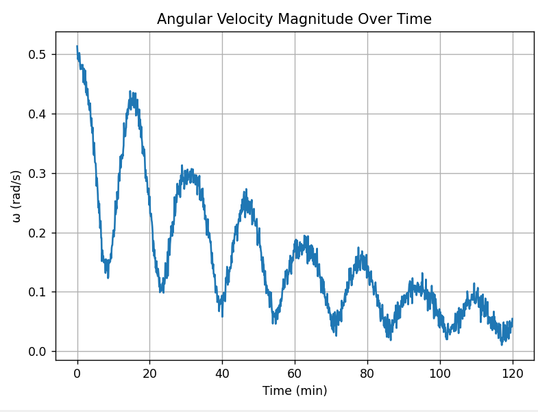
<p class="text-center" style="font-size:0.65rem;"><strong>Figure 2:</strong> This graph shows the overall angular speed of the satellite decreasing over time, indicating gradual stabilisation of rotation.</p>

<p>The angular velocity $ |\boldsymbol{\omega}(t)| $ gradually decays and oscillates with decreasing amplitude. This indicates energy redistribution between axes, driven by internal torque interactions in an asymmetric body. Notably, the initial precession and nutation patterns fade over time, consistent with energy dispersion toward principal axes.</p>

<h3 id="2-angular-acceleration-magnitude-over-time">2. Angular Acceleration Magnitude Over Time</h3>

<p align="center">
  <img src="/assets/images/angular_acceleration_magnitude.png" alt="Angular Acceleration Magnitude" style="max-width:100%;" />
</p>
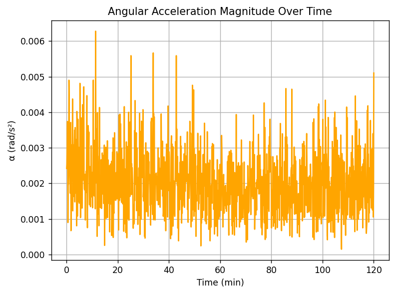
<p class="text-center" style="font-size:0.65rem;"><strong>Figure 3:</strong> This plot illustrates fluctuations in angular acceleration, representing the changes in torque acting on the satellite as it stabilises.</p>

<p>Angular acceleration $ |\dot{\boldsymbol{\omega}}(t)| $ remains low in magnitude, reflecting the lack of external torque input. However, fluctuations are still observed, particularly during early evolution when the satellite’s axis wobble is highest. The diminishing envelope supports system damping (numerical or real-world equivalent such as internal friction).</p>

<h3 id="3-rotational-kinetic-energy-over-time">3. Rotational Kinetic Energy Over Time</h3>

<p align="center">
  <img src="/assets/images/rotational_kinetic_energy.png" alt="Rotational Kinetic Energy" style="max-width:100%;" />
</p>
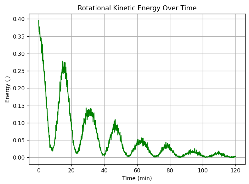
<p class="text-center" style="font-size:0.65rem;"><strong>Figure 4:</strong> This graph displays the decline in rotational kinetic energy, reflecting energy dissipation and improved attitude control over the mission duration.</p>

<p>The satellite’s rotational kinetic energy $ KE(t) $ declines in a stepwise oscillatory pattern, consistent with energy transfer between rotational modes. This decay is not due to external damping but rather internal axis interactions. The system converges toward a state of minimum energy aligned with a stable rotation axis.</p>

<p>These behaviours qualitatively match predictions from rigid body dynamics and past case studies of free tumbling satellites (e.g., Explorer 1).</p>

<h2 id="evaluation">Evaluation</h2>

<p>The simulation faithfully captures the nonlinear dynamics of a free rigid body in space, including precession, nutation, and stabilisation behaviour. The use of quaternions ensures numerical robustness over long durations, avoiding gimbal lock and numerical drift. The results are realistic and consistent with expected physical principles, particularly:</p>

<ul>
  <li>Conservation of angular momentum.</li>
  <li>Oscillatory transitions as energy is redistributed.</li>
  <li>Long-term convergence toward a stable rotational state.</li>
</ul>

<p>There are, however, simplifications:</p>
<ul>
  <li>The model assumes perfect rigidity with no internal damping.</li>
  <li>There are no external torques (e.g., gravity gradient, solar pressure).</li>
  <li>No active control mechanisms are simulated.</li>
</ul>

<p>Nonetheless, the simulation offers valuable insights into passive stability regimes and can be extended to include perturbative torques or active control systems.</p>

<h2 id="conclusion">Conclusion</h2>

<p>This project demonstrates the utility of physics-based simulation in modelling satellite attitude dynamics. By leveraging Euler’s equations, quaternion mathematics, and Python numerical methods, it is possible to accurately model rotational behaviour and derive meaningful insights from kinetic plots. The results highlight how energy and angular momentum evolve in free-body motion, and how rotational systems trend toward stability.</p>

<p>Future extensions could include:</p>
<ul>
  <li>Magnetorquer or reaction wheel control.</li>
  <li>Perturbation modelling (gravity gradient torque, SRP).</li>
  <li>Kalman filtering for state estimation.</li>
</ul>

<p>This simulation serves as a foundational model for more advanced spacecraft attitude control simulations and contributes to practical understanding of free-body stabilisation dynamics in aerospace systems.</p>

<h2 id="references">References</h2>
<ul>
  <li>Sutton, G. P., &amp; Biblarz, O. (2016). Rocket Propulsion Elements (9th ed.). Wiley.</li>
  <li>Wertz, J. R. (1978). Spacecraft Attitude Determination and Control. D. Reidel Publishing Company.</li>
  <li>NASA Glenn Research Center. (n.d.). Reynolds Number. Retrieved from https://www.grc.nasa.gov/www/k-12/airplane/reynolds.html</li>
  <li>National Physical Laboratory (UK). (n.d.). Physical Constants and Units. Retrieved from https://www.npl.co.uk/</li>
  <li>Kane, T. R., Likins, P. W., &amp; Levinson, D. A. (1983). Spacecraft Dynamics. McGraw-Hill.</li>
  <li>Virtanen, P. et al. (2020). SciPy 1.0: Fundamental Algorithms for Scientific Computing in Python. Nature Methods, 17, 261–272.</li>
</ul>]]></content><author><name>James Brandt</name></author><summary type="html"><![CDATA[A Python-simulated investigation into satellite attitude stabilisation, analysing the decay of angular velocity and rotational energy over time through realistic physics-based modelling.]]></summary></entry><entry><title type="html">Aerodynamic Shape Optimisation Using Machine Learning and Evolutionary Algorithms</title><link href="https://james-brandt.github.io/aerodynamic-shape-optimisation/" rel="alternate" type="text/html" title="Aerodynamic Shape Optimisation Using Machine Learning and Evolutionary Algorithms" /><published>2025-07-15T00:00:00+10:00</published><updated>2025-07-15T00:00:00+10:00</updated><id>https://james-brandt.github.io/aerodynamic-shape-optimisation</id><content type="html" xml:base="https://james-brandt.github.io/aerodynamic-shape-optimisation/"><![CDATA[<h2 id="rationale">Rationale</h2>

<p>In mechatronic and aerospace design, aerodynamic efficiency is a critical determinant of performance, fuel consumption, and thus emissions. Minimising aerodynamic drag has been a long-term focus in engineering disciplines due to its consequences on energy efficiency and operating costs. However, manual optimisation of complex shapes remains time-consuming and limited by human intuition.</p>

<p>This project investigates the utilisation of evolutionary algorithms to autonomously optimise a three-dimensional axisymmetric object’s geometry to reduce its aerodynamic drag. By simulating 1000 generations of Differential Evolution followed by 1000 iterations of Covariance Matrix Adaptation Evolution Strategy (CMA-ES), the programme aims to refine shapes using physics-informed fitness evaluations. The objective of this programme is to demonstrate the applicability of machine learning in solving real-world engineering problems involving fluid dynamics, stability, and form efficiency.</p>

<h2 id="background-information">Background Information</h2>

<h3 id="aerodynamic-drag">Aerodynamic Drag</h3>

<p>Drag is the resistance force acting opposite to the motion of an object moving through a fluid, such as air. It is composed of several components:</p>

<ul>
  <li><strong>Form Drag (Pressure Drag)</strong> arises from the shape of the object and the pressure differential between the front and rear surfaces.</li>
  <li><strong>Skin Friction Drag</strong> is caused by viscous shear stresses in the boundary layer of air along the surface.</li>
  <li><strong>Base Drag</strong> occurs at the rear of bluff bodies due to flow separation.</li>
  <li><strong>Induced Drag</strong> arises from lift generation, albeit minimal for streamlined bodies.</li>
  <li><strong>Wake Drag</strong> is associated with turbulence behind the object.</li>
</ul>

<p>These drag forces are typically modelled using:</p>

\[D = \frac{1}{2} \rho v^2 C_d A\]

<p>Where:</p>

<ul>
  <li>$D$ is the drag force (N)</li>
  <li>$\rho$ is the air density (kg/m³)</li>
  <li>$v$ is the velocity (m/s)</li>
  <li>$C_d$ is the drag coefficient (dimensionless)</li>
  <li>$A$ is the frontal area (m²)</li>
</ul>

<h3 id="reynolds-number">Reynolds Number</h3>

<p>The Reynolds number, given by:</p>

\[Re = \frac{\rho v L}{\mu}\]

<p>quantifies the flow regime, separating laminar and turbulent conditions. The critical Reynolds number of $5 \times 10^5$ is used to switch between laminar and turbulent skin friction formulations.</p>

<h3 id="evolutionary-algorithms">Evolutionary Algorithms</h3>

<p>Evolutionary algorithms are heuristic optimisation techniques inspired by natural selection. Two methods are used in this study:</p>

<ul>
  <li><strong>Differential Evolution (DE)</strong> iteratively evolves a population of candidate solutions by combining existing candidates to generate new ones, selecting those with better performance.</li>
  <li><strong>CMA-ES</strong> (Covariance Matrix Adaptation Evolution Strategy) refines solutions by sampling from a multivariate Gaussian distribution and updating its covariance matrix based on successful solutions.</li>
</ul>

<p>These algorithms require an objective function to evaluate each solution, in this case, total aerodynamic drag.</p>

<h3 id="geometry-modelling">Geometry Modelling</h3>

<p>The object is defined by a set of control points describing half of its side profile. These points are interpolated using cubic splines. The resulting profile is revolved to estimate frontal area, wetted area, and volume. The shape is then assessed based on fluid dynamic parameters.</p>

<h3 id="additional-physics">Additional Physics</h3>

<p>The simulation incorporates additional physical phenomena:</p>
<ul>
  <li><strong>Compressibility Corrections</strong> for Mach numbers above 0.3 using the Prandtl-Glauert transformation.</li>
  <li><strong>Stability Margins</strong> calculated using an estimate of the centre of mass and centre of pressure.</li>
  <li><strong>Ground Effect</strong> reduces form drag when near the surface.</li>
  <li><strong>Surface Roughness</strong> adds a correction factor to simulate real-world conditions.</li>
</ul>

<h2 id="methodology">Methodology</h2>

<h3 id="constants-and-assumptions">Constants and Assumptions</h3>

<p>The following constants and assumptions were applied:</p>
<ul>
  <li>Velocity: 30 m/s</li>
  <li>Target Mass: 500 kg</li>
  <li>Max Side Profile Length: 3.0 m</li>
  <li>Max Frontal Profile Length: 1.0 m</li>
  <li>Object Density: 500 kg/m³</li>
  <li>Air density: 1.225 kg/m³ (at sea level)</li>
  <li>Surface roughness coefficient: 1.05</li>
  <li>Lift coefficient: 0.05 (to simulate mild induced drag)</li>
  <li>Ground effect applied below 0.5 m altitude</li>
</ul>

<h3 id="simulation-procedure">Simulation Procedure</h3>

<p>The simulation proceeds as follows:</p>

<p><strong>1. Initial Geometry Generation:</strong></p>

<div class="language-python highlighter-rouge"><div class="highlight"><pre class="highlight"><code><span class="k">def</span> <span class="nf">generate_profile</span><span class="p">(</span><span class="n">control_points</span><span class="p">,</span> <span class="n">length</span><span class="p">,</span> <span class="n">num_points</span> <span class="o">=</span> <span class="mi">500</span><span class="p">):</span>
    <span class="n">xs_control</span> <span class="o">=</span> <span class="n">np</span><span class="p">.</span><span class="n">linspace</span><span class="p">(</span><span class="mi">0</span><span class="p">,</span> <span class="n">length</span><span class="p">,</span> <span class="n">NUM_CONTROL_POINTS</span><span class="p">)</span>
    <span class="n">ys_control</span> <span class="o">=</span> <span class="n">np</span><span class="p">.</span><span class="nb">abs</span><span class="p">(</span><span class="n">control_points</span><span class="p">)</span>
    <span class="n">ys_control</span><span class="p">[</span><span class="mi">0</span><span class="p">]</span> <span class="o">=</span> <span class="n">ys_control</span><span class="p">[</span><span class="o">-</span><span class="mi">1</span><span class="p">]</span> <span class="o">=</span> <span class="mi">0</span>
    <span class="n">interp_func</span> <span class="o">=</span> <span class="n">interp1d</span><span class="p">(</span><span class="n">xs_control</span><span class="p">,</span> <span class="n">ys_control</span><span class="p">,</span> <span class="n">kind</span> <span class="o">=</span> <span class="s">"cubic"</span><span class="p">)</span>
    <span class="n">xs</span> <span class="o">=</span> <span class="n">np</span><span class="p">.</span><span class="n">linspace</span><span class="p">(</span><span class="mi">0</span><span class="p">,</span> <span class="n">length</span><span class="p">,</span> <span class="n">num_points</span><span class="p">)</span>
    <span class="n">ys</span> <span class="o">=</span> <span class="n">interp_func</span><span class="p">(</span><span class="n">xs</span><span class="p">)</span>
    <span class="k">return</span> <span class="n">xs</span><span class="p">,</span> <span class="n">ys</span>
</code></pre></div></div>

<p>The ML algorithm modifies the shape by adjusting a vector of parameters that includes:</p>
<ul>
  <li>Eight vertical control point values, which define the curvature of the side profile using cubic spline interpolation. These values control the local radius along the object’s length, effectively shaping the profile’s smoothness, thickness distribution, and taper.</li>
  <li>Total side profile length, which determines the overall body length of the shape and influences the fineness ratio.</li>
  <li>Frontal profile length (width), which defines the elliptical diameter of the object’s cross-section and directly affects the frontal area.</li>
</ul>

<p>These twelve parameters allow the ML algorithm to explore a wide design space of slender, symmetrical bodies while ensuring that the shape remains smooth and physically realistic. Although, the three-dimensional shape remains incredibly rudimentary when compared to the real-world applications of drag reduction.</p>

<p><strong>2. Drag Evaluation:</strong>
The main function computes:</p>
<ul>
  <li>Frontal and wetted surface area.</li>
  <li>Reynolds number and skin friction.</li>
  <li>Volume and mass penalties.</li>
  <li>Smoothness and stability penalties.</li>
  <li>Total drag (sum of all components).</li>
</ul>

<div class="language-python highlighter-rouge"><div class="highlight"><pre class="highlight"><code><span class="k">def</span> <span class="nf">evaluate_drag</span><span class="p">(</span><span class="n">params</span><span class="p">,</span> <span class="n">velocity</span><span class="p">,</span> <span class="n">target_mass</span><span class="p">):</span>
    <span class="p">...</span>
</code></pre></div></div>

<p><strong>3. Optimisation:</strong></p>
<ul>
  <li>Differential Evolution runs for 1000 generations.</li>
  <li>CMA-ES uses the DE result as a seed and performs 1000 iterations.</li>
</ul>

<div class="language-python highlighter-rouge"><div class="highlight"><pre class="highlight"><code><span class="n">result_de</span> <span class="o">=</span> <span class="n">differential_evolution</span><span class="p">(...)</span>
<span class="n">es</span> <span class="o">=</span> <span class="n">cma</span><span class="p">.</span><span class="n">CMAEvolutionStrategy</span><span class="p">(</span><span class="n">result_de</span><span class="p">.</span><span class="n">x</span><span class="p">.</span><span class="n">tolist</span><span class="p">(),</span> <span class="mf">0.02</span><span class="p">)</span>
<span class="n">es</span><span class="p">.</span><span class="n">optimize</span><span class="p">(</span><span class="k">lambda</span> <span class="n">p</span><span class="p">:</span> <span class="n">evaluate_drag</span><span class="p">(</span><span class="n">p</span><span class="p">,</span> <span class="n">velocity</span><span class="p">,</span> <span class="n">target_mass</span><span class="p">,</span> <span class="n">max_length</span><span class="p">,</span> <span class="n">max_front_length</span><span class="p">),</span> <span class="n">iterations</span> <span class="o">=</span> <span class="mi">1000</span><span class="p">)</span>
</code></pre></div></div>

<p><strong>4. Logging and Visualisation:</strong>
Each generation’s data is stored in a DataFrame and visualised through:</p>
<ul>
  <li>Side and frontal profile plots, to determine the accuracy of the programme.</li>
  <li>Drag versus generation graph, to investigate the impact of each subsequent generation on drag.</li>
</ul>

<h2 id="results-analysis">Results Analysis</h2>

<h3 id="final-output">Final Output</h3>

<p>After 2000 total optimisation steps (1000 DE + 1000 CMA-ES), the best solution appeared in Generation 990.</p>

<table>
  <thead>
    <tr>
      <th>Parameter</th>
      <th>Value</th>
    </tr>
  </thead>
  <tbody>
    <tr>
      <td>Generation</td>
      <td>990</td>
    </tr>
    <tr>
      <td>Final Drag (N)</td>
      <td>169.21</td>
    </tr>
    <tr>
      <td>Velocity (m/s)</td>
      <td>30.0</td>
    </tr>
    <tr>
      <td>Mass (kg)</td>
      <td>500.0</td>
    </tr>
    <tr>
      <td>Length (m)</td>
      <td>3.0</td>
    </tr>
    <tr>
      <td>Frontal Width (m)</td>
      <td>0.77</td>
    </tr>
    <tr>
      <td>Frontal Length (m)</td>
      <td>1.0</td>
    </tr>
  </tbody>
</table>

<p class="text-center" style="font-size:0.65rem;">
  <strong>Table 1:</strong> Fully optimised parameters of the shape at its most optimal generation.
</p>

<p align="center">
  <img src="/assets/images/final_profile.jpg" alt="Final Profile" style="max-width:100%;" />
</p>
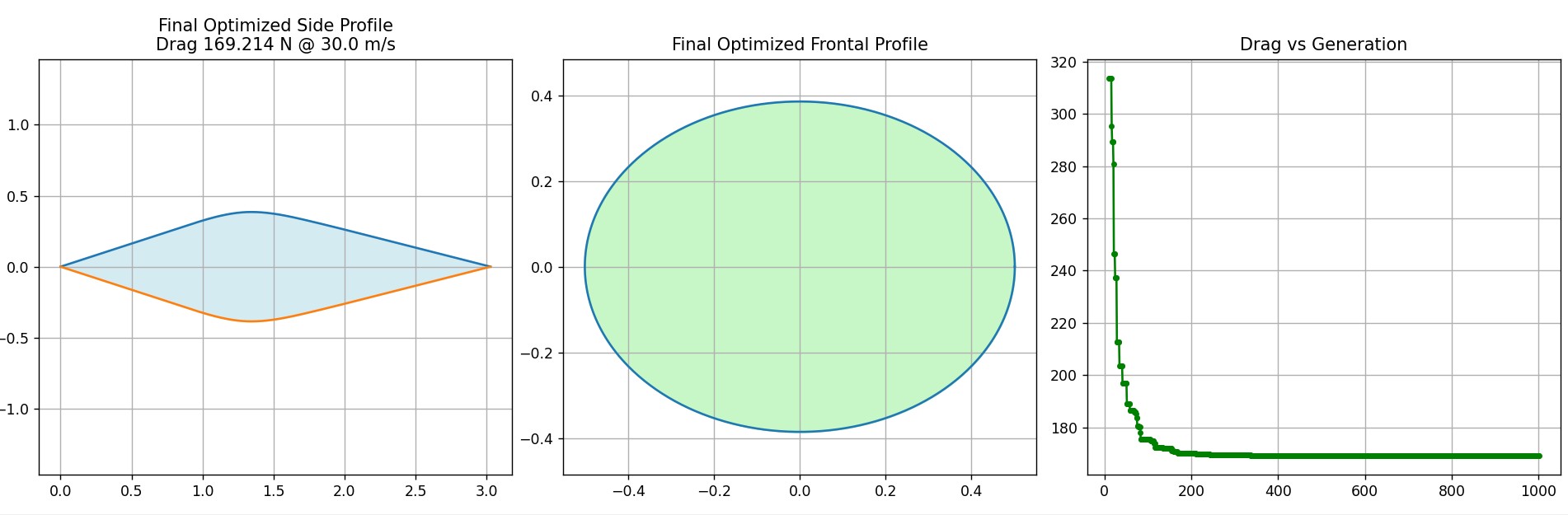
<p class="text-center" style="font-size:0.65rem;"><strong>Figure 1:</strong> Final profile of optimised shape showing smooth axisymmetric curvature, and a graph displaying the change in drag over each generation.</p>

<p align="center">
  <video controls="" autoplay="" loop="" muted="" playsinline="" style="max-width:100%;">
    <source src="/assets/videos/shape_evolution.mp4" type="video/mp4" />
    Your browser does not support the video tag.
  </video>
</p>
<p class="text-center" style="font-size:0.65rem;"><strong>Figure 2:</strong> Drag evolution over 1000 generations of Differential Evolution and CMA-ES.</p>

<h3 id="side-and-frontal-profile">Side and Frontal Profile</h3>

<p>The final side profile exhibits a smooth, continuous curvature that peaks at the midsection and tapers symmetrically towards the nose and tail (a symmetrical teardrop shape). This streamlined geometry minimises pressure drag by delaying flow separation, particularly at higher velocities where adverse pressure gradients are more influential. The use of cubic spline interpolation across eight control points ensures a high degree of shape control without introducing abrupt surface changes, which would otherwise elevate form drag.</p>

<p>The frontal profile is elliptical, a shape known to reduce stagnation pressure at the leading edge while also constraining frontal area. This elliptical cross-section balances structural efficiency and aerodynamic performance, producing a compact footprint (0.7707 m diameter) relative to the overall length (3.0 m). Note that the frontal profile is a 2-dimensional representation of how the shape would appear from the front, thus displaying the shape’s largest surface area from the frontal plane.</p>

<p>Together, these forms suggest a high fineness ratio design that is representative of real-world applications such as drop tanks, unmanned aerial vehicles, or missile fuselages, where low drag and dynamic stability are critical.</p>

<h3 id="drag-vs-generation">Drag vs Generation</h3>

<p>As the number of generations increases from 0 to 50, the drag decreases significantly in decreasing increment, which is due to the elimination of grossly inefficient shapes early on. Subsequent refinements were smaller, with diminishing returns as the algorithms approached local minima. Onwards from generation 50, the data displays an inverse proportionality, as the drag decreases negligibly and plateaus. From here, the CMA-ES began optimisation within an already narrow solution space.</p>

<p>This behaviour reflects a realistic optimisation curve, where coarse improvements precede subtle, high-fidelity tuning. Evidently, only 400 generations are necessary for a decently accurate drag reduction to occur, but extremely precise operations may require more. Importantly, skipping the first five generations from the plot improves readability by excluding early-stage outliers.</p>

<h2 id="evaluation">Evaluation</h2>

<h3 id="accuracy-and-limitations">Accuracy and Limitations</h3>

<ul>
  <li>The drag models are simplified, lacking vortex shedding, turbulent wake prediction, or 3D finite element resolution.</li>
  <li>Revolved axisymmetric bodies do not capture features like wings, vents, or sharp edges.</li>
  <li>No structural or thermal constraints were considered beyond stability margins.</li>
  <li>Air density remains fixed, without altitude or temperature variation beyond a single exponential decay.</li>
</ul>

<h3 id="suggested-improvements">Suggested Improvements</h3>

<ol>
  <li>Incorporate Real CFD Libraries such as OpenFOAM or PyFoam for detailed pressure field evaluation.</li>
  <li>Thermal Constraints to simulate high-speed heating or radiative cooling.</li>
  <li>Material Strength Models to introduce minimum wall thickness or failure stress constraints.</li>
  <li>Stochastic Wind Conditions to evaluate shape performance under varying angles of attack or gusts.</li>
  <li>Multifidelity Models where rough analytical models guide early optimisation, switching to CFD later.</li>
</ol>

<h2 id="conclusion">Conclusion</h2>

<p>This project demonstrated the employment of evolutionary algorithms to optimise a superficial three-dimensional shape for minimal aerodynamic drag. By integrating mathematical modelling, physics-based penalty functions, and machine learning-based search, the program effectively identified efficient geometries under realistic constraints. The success of this approach in a simplified domain provides a valuable stepping stone toward more sophisticated design tools in aerospace, automotive, and civil engineering contexts. Continued development, particularly through integration with CFD and real-world testing, would significantly enhance the fidelity and applicability of such simulations.</p>

<h2 id="references">References</h2>

<ul>
  <li>Anderson, J. D. (2010). <em>Fundamentals of Aerodynamics</em>. McGraw-Hill.</li>
  <li>Hansen, N. (2006). <em>The CMA Evolution Strategy: A Comparing Review</em>.</li>
  <li>White, F. M. (2011). <em>Fluid Mechanics</em>. McGraw-Hill.</li>
  <li>NASA Glenn Research Center. (2022). <em>Drag Equation</em>. <a href="https://www.grc.nasa.gov">https://www.grc.nasa.gov</a></li>
</ul>]]></content><author><name>James Brandt</name></author><summary type="html"><![CDATA[Using evolutionary algorithms and simulation-based modelling to reduce aerodynamic drag through shape refinement and optimisation techniques.]]></summary></entry></feed>